TCP Congestion Control & Flow Control Mechanics: Sliding Windows, CUBIC, and BBR

At the transport layer of modern IP networks, the Transmission Control Protocol (TCP) guarantees reliable, in-order byte stream delivery over inherently lossy and uncoordinated packet-switched channels. While byte sequence numbers, checksums, and acknowledgement (ACK) flags ensure data integrity, TCP’s true operational complexity lies in its dynamic rate-regulation algorithms: flow control and congestion control.

A common point of confusion in network engineering is the distinction between these two rate-limiting mechanisms:

Flow Control: Prevents a fast sender from overwhelming a slow receiver’s processing buffer.
Congestion Control: Prevents a group of competing senders from overwhelming intermediate network bottlenecks, router buffers, and switching fabrics.

In this guide, we analyze the mathematical foundations and kernel implementation of TCP transmission mechanics. We explore sliding window state pointers, receive window scaling (RFC 7323), classic loss-based congestion control algorithms (Reno and CUBIC), model-based bandwidth estimation (BBR), and practical Linux kernel sysctl performance tuning.

1. TCP Flow Control & The Sliding Window Architecture

TCP flow control relies on a sliding window mechanism. Instead of transmitting a single segment and waiting for an individual ACK before sending the next—which would reduce throughput to a fraction of available capacity on high-latency links—TCP allows the sender to transmit multiple bytes up to a dynamically advertised limit.

Receiver-Advertised Window ($rwnd$)

Every TCP header contains a 16-bit Window Size field. The advertised Receive Window ($rwnd$) is derived from the currently available space in the receiver’s TCP socket receive buffer. In Linux, the total allocated memory limit for a socket’s receive queue is represented by sk_rcvbuf (managed by kernel autotuning via tcp_moderate_rcvbuf), while $rwnd$ reflects the subset of this buffer currently available for incoming application payload data:

$$\text{Free Buffer Space} = \text{Buffer}{\text{max}} - (\text{Bytes}{\text{received}} - \text{Bytes}_{\text{read_by_app}})$$

The receiver writes this value into the TCP header as the Receive Window ($rwnd$). If the application consuming the socket halts or executes slowly, $rwnd$ decreases. If the receive buffer fills completely, the receiver advertises $rwnd = 0$, halting further transmission until the buffer drains.

Sender Buffer Pointers

The TCP sender maintains a byte-array buffer tracked by four state pointers:

$\text{SND.UNA}$ (Send Unacknowledged): The sequence number of the oldest unacknowledged byte.
$\text{SND.NXT}$ (Send Next): The sequence number of the next byte to be transmitted.
$\text{SND.WND}$ (Send Window): The maximum size of the transmission window.
$\text{SND.WL1}$ / $\text{SND.WL2}$: Sequence and acknowledgement numbers used to update the send window.

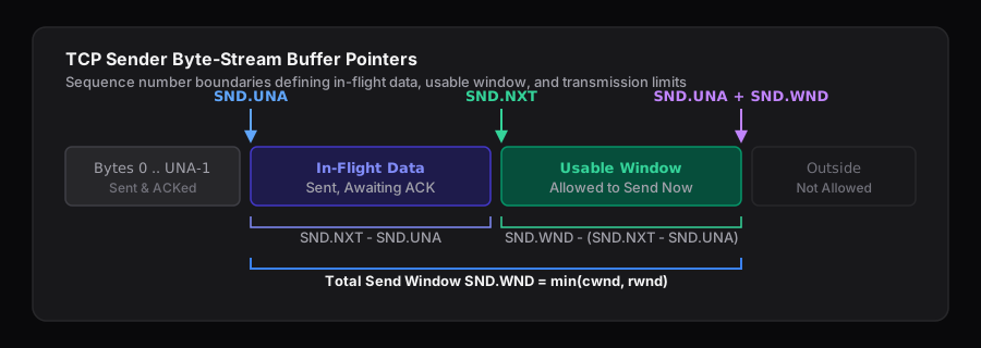
TCP Sender Byte-Stream Buffer Pointers

The sender calculates its Usable Window—the exact number of additional bytes it can transmit immediately—using:

$$\text{Usable Window} = \text{SND.WND} - (\text{SND.NXT} - \text{SND.UNA})$$

2. Window Scaling & The Bandwidth-Delay Product (BDP)

The standard TCP header allocates 16 bits for the Window Size field, capping the maximum advertised receive window at $2^{16} - 1 = 65,535\text{ bytes}$ (64 KB).

On local area networks with sub-millisecond latency, a 64 KB window is often sufficient. However, on long-haul optical routes or high-throughput cloud links, a 64 KB limit severely throttles throughput.

Bandwidth-Delay Product Math

The maximum theoretical volume of unacknowledged data required to fully saturate a network pipe is defined by the Bandwidth-Delay Product (BDP):

$$\text{BDP} = \text{Link Bandwidth} \times \text{Round-Trip Time (RTT)}$$

For detailed latency component breakdowns and interactive BDP calculations, refer to the Network Latency Calculator and our overview of Network Latency Mechanics.

Consider a 10 Gbps transatlantic link with an RTT of 80 ms:

$$\text{BDP} = (10 \times 10^9 \text{ bits/sec}) \times (0.080 \text{ sec}) = 800,000,000 \text{ bits} = 100 \text{ MB}$$

If the TCP window is constrained to the legacy 64 KB limit, the maximum achievable throughput is bounded by:

$$\text{Max Throughput} = \frac{\text{Window Size}}{\text{RTT}} = \frac{65,535 \times 8 \text{ bits}}{0.080 \text{ sec}} \approx 6.55 \text{ Mbps}$$

Despite operating over a 10 Gbps channel, the connection utilizes less than 0.1 percent of available capacity due to window exhaustion.

TCP Window Scale Option (RFC 7323)

To overcome this constraint, RFC 7323 defines the TCP Window Scale option negotiated during the initial three-way handshake (SYN and SYN-ACK segments). The negotiated window scale factor is exchanged exclusively during this initial handshake and remains fixed for the lifetime of the connection.

The option specifies a 1-byte scale factor ($S \le 14$). The actual effective receive window is computed by left-shifting the 16-bit header value by $S$ bits:

$$\text{Effective } rwnd = \text{Header Window Value} \times 2^S$$

With a maximum shift factor of 14, the maximum achievable window size expands to:

$$\text{Max Window} = 65,535 \times 2^{14} = 1,073,725,440\text{ bytes} \approx 1\text{ GB}$$

3. TCP Congestion Control Mechanics

While flow control is governed by the receiving host, congestion control is executed by the sending host to prevent intermediate routers from dropping packets due to queue overflow.

To achieve this, the sender maintains a second window variable: the Congestion Window ($cwnd$). The maximum volume of unacknowledged in-flight data is strictly bounded by the smaller of the two windows:

$$\text{Effective Transmission Limit } W = \min(cwnd, rwnd)$$

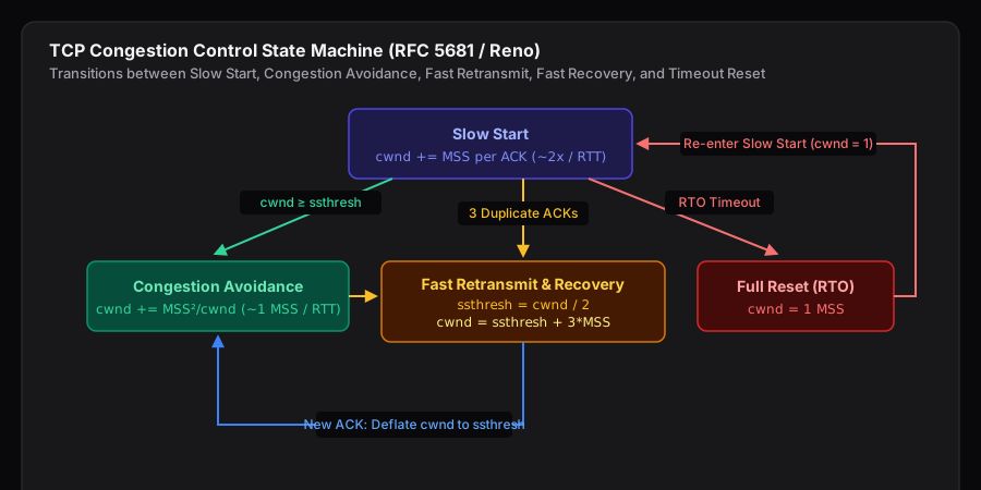
Classical TCP congestion control operates as a feedback loop structured into distinct operational phases defined in RFC 5681: Slow Start, Congestion Avoidance, Fast Retransmit, and Fast Recovery.

TCP Congestion Control State Machine

Phase 1: Slow Start

When a connection is established, the sender has no prior knowledge of the network topology or bottleneck link capacity. Rather than flooding the network immediately, the sender initializes $cwnd$ to a conservative value (typically 10 Maximum Segment Sizes (MSS) per RFC 6928, or approximately 14,600 bytes).

During Slow Start, for each ACK acknowledging new data, $cwnd$ increases by up to 1 MSS. While delayed ACKs may acknowledge multiple segments in a single cumulative response, modern TCP stack implementations (utilizing mechanisms such as Appropriate Byte Counting, RFC 3465) scale window expansion based on the number of previously unacknowledged bytes delivered. As a result, $cwnd$ achieves approximately exponential growth per RTT under normal operational conditions:

$$\Delta cwnd = \text{MSS} \quad \text{(per ACK acknowledging new data)}$$

$$cwnd(t + \text{RTT}) \approx 2 \cdot cwnd(t)$$

Exponential expansion continues until one of two threshold events occurs:

$cwnd$ reaches the Slow Start Threshold ($ssthresh$).
A loss event occurs (via duplicate ACKs or retransmission timeout).

Phase 2: Congestion Avoidance (AIMD)

When $cwnd \ge ssthresh$, the protocol transitions to Congestion Avoidance to probe for extra bandwidth linearly rather than exponentially. Classic TCP Reno uses Additive Increase Multiplicative Decrease (AIMD):

Additive Increase: For each full RTT without loss, $cwnd$ grows by approximately 1 MSS. Per ACK acknowledging new data during congestion avoidance, $cwnd$ increases according to the conventional form:

$$\Delta cwnd = \frac{\text{MSS}^2}{cwnd}$$

This can also be expressed as $\Delta cwnd = \text{MSS} \times \frac{\text{MSS}}{cwnd}$, yielding an aggregate increase of approximately 1 MSS per RTT.

Multiplicative Decrease: Upon detecting packet loss, the network signals congestion. The sender halves the slow-start threshold and reduces $cwnd$:

$$ssthresh = \frac{cwnd}{2}, \quad cwnd = ssthresh$$

Phase 3: Fast Retransmit and Fast Recovery

Earlier TCP implementations relied solely on the Retransmission Timeout (RTO) timer to detect dropped packets. When an RTO timer expires, the sender assumes severe network failure, drops $cwnd$ to 1 MSS, and re-enters Slow Start, causing severe throughput penalties.

Modern implementations use Fast Retransmit:

If a single segment is lost in a stream, subsequent out-of-order arrivals cause the receiver to send duplicate ACKs referencing the last in-order sequence number.
Upon receiving 3 duplicate ACKs, the sender infers packet loss without waiting for the RTO timer to expire.
The sender immediately retransmits the missing segment (Fast Retransmit) and enters Fast Recovery:
- Sets $ssthresh = \frac{cwnd}{2}$.
- Inflates $cwnd = ssthresh + 3 \times \text{MSS}$ to account for buffered segments that have left the network.
- Resumes linear growth once the missing segment is fully acknowledged and $cwnd$ is deflated back to $ssthresh$.

4. Modern Loss-Based vs. Model-Based Algorithms: CUBIC and BBR

Classic AIMD works effectively on low-speed networks, but scales poorly on high-bandwidth, high-latency links (often termed long-fat networks). Modern Linux deployments rely on advanced algorithms optimized for distinct bottleneck behaviors.

TCP CUBIC (Linux Default)

TCP CUBIC (RFC 8312) replaces linear window growth with a cubic function dependent on elapsed time $t$, where $t$ represents the elapsed time within the current congestion avoidance epoch (following the last congestion event). While upstream Linux defaults to TCP CUBIC, many cloud providers and high-throughput edge networks deploy BBR as their primary congestion control algorithm.

$$W_{\text{cubic}}(t) = C \cdot (t - K)^3 + W_{\text{max}}$$

Where:

$W_{\text{max}}$ is the window size immediately before the last congestion event.
$C$ is a scaling constant.
$K$ is the time period required for the window to grow back to $W_{\text{max}}$ in the absence of further congestion:

$$K = \sqrt[3]{\frac{W_{\text{max}} \cdot \beta}{C}}$$

where $\beta$ is the multiplicative decrease factor.

TCP CUBIC Growth Curve

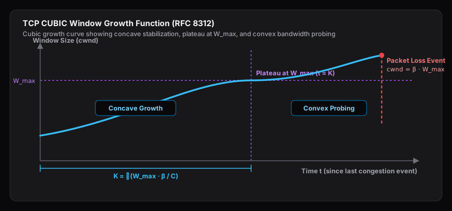
The cubic function provides two primary performance benefits:

Stabilization: As $t$ approaches $K$, window growth flattens, stabilizing near $W_{\text{max}}$ to maintain steady link saturation.
Aggressive Probing: Once $t > K$, window expansion accelerates cubically to discover newly freed bandwidth across gigabit and multi-gigabit pipes.

BBR: Bottleneck Bandwidth and RTT

Both Reno and CUBIC are loss-based algorithms. They assume that packet loss is a direct indicator of network congestion. However, in modern networks equipped with oversized router buffers (bufferbloat), loss-based algorithms fill intermediate queues to capacity before dropping a single packet. This creates hundreds of milliseconds of artificial queuing latency without increasing link throughput.

BBR (Bottleneck Bandwidth and RTT), developed by Google, is a model-based congestion control algorithm. BBR continuously samples packet delivery rates to build an explicit model of the physical pipe:

$\text{BtlBW}$ (Bottleneck Bandwidth): The maximum delivery rate observed over a moving time window.
$\text{RTprop}$ (Round-Trip Propagation Delay): The minimum RTT observed without queuing delay.

BBR targets an operating point centered around the estimated physical Bandwidth-Delay Product:

$$\text{Target Inflight} = \text{BtlBW} \times \text{RTprop}$$

Rather than maintaining a static or exact BDP-sized flight at all times, BBR operates across four primary state machine phases (STARTUP, DRAIN, PROBE_BW, and PROBE_RTT). It periodically probes above its estimated bandwidth during PROBE_BW (to discover newly available capacity) and below it in DRAIN or PROBE_RTT (to drain standing queue accumulation and accurately re-measure minimum propagation delay). This model-based control achieves maximum bottleneck throughput while suppressing bufferbloat.

5. Linux Kernel Network Tuning & Sysctl Configuration

In production backend environments, achieving optimal throughput across high-capacity interfaces requires tuning Linux kernel socket buffers and congestion control modules via /etc/sysctl.conf.

1. Memory Buffer Allocation (`tcp_rmem` & `tcp_wmem`)

Linux dynamically tunes socket memory buffers based on link conditions. System administrators define buffer limits via three-element vectors representing [min, default, max] memory in bytes:

# Allocate up to 16MB for receive and transmit buffers on high-BDP links
net.ipv4.tcp_rmem = 4096 87380 16777216
net.ipv4.tcp_wmem = 4096 65536 16777216

Ensure global network memory limits (net.core.rmem_max and net.core.wmem_max) match or exceed the maximum socket buffer thresholds:

net.core.rmem_max = 16777216
net.core.wmem_max = 16777216

2. Window Scaling and Timestamps

Verify that window scaling (RFC 7323) and selective acknowledgements (SACK, RFC 2018) are enabled:

net.ipv4.tcp_window_scaling = 1
net.ipv4.tcp_sack = 1
net.ipv4.tcp_timestamps = 1

SACK allows receivers to acknowledge non-contiguous block ranges during packet loss, permitting senders to retransmit missing segments without retransmitting data that has already arrived safely.

TCP Timestamps (net.ipv4.tcp_timestamps = 1, RFC 7323) provide high-precision Round-Trip Time Measurement (RTTM) for accurate RTO estimation and enable Protection Against Wrapped Sequence Numbers (PAWS), which prevents stale or delayed segments from corrupting high-throughput connections on gigabit and multi-gigabit links.

3. Switching Congestion Control Modules to BBR

To check available congestion control modules in the current kernel:

sysctl net.ipv4.tcp_available_congestion_control
# Output: net.ipv4.tcp_available_congestion_control = reno cubic bbr

To configure BBR as the default congestion control algorithm alongside the Fair Queueing (fq) packet scheduler:

net.core.default_qdisc = fq
net.ipv4.tcp_congestion_control = bbr

Note that fq (Fair Queueing) is the strongly recommended queuing discipline for TCP pacing under BBR, although modern Linux kernels can also provide socket-level pacing with other queuing disciplines (such as fq_codel).

Apply parameters dynamically without rebooting:

sudo sysctl -p

# Or reload configuration across all /etc/sysctl.d/*.conf system files:
sudo sysctl --system

On modern Linux distributions where configuration parameters are modularized across /etc/sysctl.d/, sudo sysctl --system is preferred over sysctl -p.

6. Architectural Summary & Cross-Domain Considerations

Understanding TCP transmission mechanics is essential when designing load-balanced application tiers, configuring edge ingress proxies, and isolating network performance bottlenecks:

Parameter / Feature	TCP Flow Control	TCP Congestion Control
Primary Scope	End-to-end endpoint buffer constraint	Intermediate network link capacity constraint
Governing Variable	Receive Window ($rwnd$)	Congestion Window ($cwnd$)
Determining Host	Receiver (advertised in TCP header)	Sender (calculated via ACK timing & loss)
Primary Risk Managed	Receiver socket buffer overflow	Router bufferbloat & packet drop storms
Key Standards	RFC 7323 (Window Scale)	RFC 5681, RFC 8312 (CUBIC), BBR

For edge architectures employing layer 4 or layer 7 proxies, connection termination splits TCP loops into two independent segments (client-to-proxy and proxy-to-upstream). For further analysis of proxy architecture and load balancer routing mechanics, see our engineering guide on Layer 4 vs Layer 7 Load Balancing and network perimeter design in Subnetting and CIDR Notation.